3D Gaussian Splatting for Real-Time Radiance Field Rendering

---

Backgrounds

1. Anisotropic（各向异性的） 3D Gaussians
2. Splatting Method（抛雪球法）
3. Tiling（数据分块）

Background 01: Anisotropic（各向异性的） 3D Gaussians

$G(\mathbf x)=\exp\big(-\frac{1}{2}(\mathbf x)^T\Sigma^{-1}(\mathbf x)\big)$

• “位置”用均值 $\mathbf \mu$ 来刻画
• “形状”用 3D 协方差矩阵 $\Sigma$ 来刻画

Background 02： Splatting Method（抛雪球法）

• 把 Fields 中每个 Voxel（Point）看作一个“能量源“
• 每个 Voxel 向图像平面投影
• 用以 Voxel 的投影点为中心的重建核将体素的“能量”“扩散”到图像像素上。
  • 在这篇论文里，其“重建核”是 3D Gaussian Function

Background 03： Tiling（数据分块）

• GPU 上各种内存的访问速度为：
  • $\text{Global memory} << \text{Shared memory} < \text{Register}$
• Global memory 大而慢， Shared memory 小而快
• 减少内存访问延迟的一个重要方向就是要尽量减少 Global memory 的访问
• 常见的策略：Tiling —— 将数据分片，然后将每个小分片缓存到 Shared Memory 中。

Motivation

• NeRFs: Implicit scene representation
  • MLP + Volumetric ray-marching
  • “is costly and can result in noise”
• 传统的 Explicit Representation
  • 优点：适合 GPU/CUDA-based rasterization
  • 缺点：传统重建方法（MVS）在场景的恢复上具有局限性（这是 Neural Rendering 的优势所在）

Overview

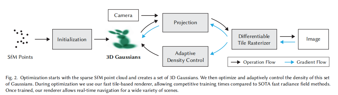
• Input: Images + Sparse Point Clouds（Generated by SFM）
• Initialize：Generate 3D Gaussian for every point
• Training：Optimization + Adaptive Density Control
• Rendering：Tile-based Rasterizer

3D Gaussian and it’s Projection

3D Gaussian 使用 $\mu$ 和 $\Sigma$ 表征： $G(\mathbf x)=\exp\big(-\frac{1}{2}(\mathbf x)^T\Sigma^{-1}(\mathbf x)\big)$

其投影变换使用一个 相机矩阵 $W$ 和其 Jacobian $J$： $\Sigma' = JW\Sigma W^TJ^T$

3D Gaussian’s Optimization

• 直接优化协方差矩阵？
  • 协方差矩阵只在半正定时才有物理意义
  • 梯度下降很难确保其有效性
• 将 $\Sigma$ 分解为 Scale Matrix $S$ 和 Rotation Matrix $R$： $\Sigma = RSS^TR^T$

优化对象

• Position $\mathbf p$
• 不透明度 $\alpha$
• 协方差 $\Sigma$
• 表征颜色的球谐函数系数 $\text{SH}$

优化方法

• 随机梯度下降
• 对于 $\alpha$ 使用 Sigmoid 激活函数
• 对于 $\Sigma$ 的 Scale 部分，使用指数激活函数
• Loss 表示为 L1 和 D-SSIM 的组合：
  • $\mathcal{L} = (1-\lambda)\mathcal{L} + \lambda\mathcal{L}_{\text{D-SSIM}}$

Adaptive Control of Gaussians

• 每 100 个 iter 进行一次密集化（Densify）
• 密集化的同时，移除 $\alpha < \epsilon_\alpha$ 的 Gauss Function

Densification Overview

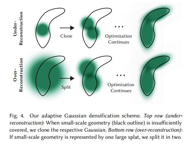
Object of Densification

• 缺失几何特征的区域（“under-reconstruction”）
• Gaussian 覆盖场景中大面积区域的情况（通常对应于”over-reconstruction”

这两种情况都具有较大的 View-space Positional Gradients。 —— 对于**梯度大于 $\tau_{\text{pos}}$ 的 Gaussian **进行密集化！

Process of Densification

• 对于 Scale 比较小的 Gaussian：
  • Clone 一份，并向梯度方向移动
• 对于 Scale 比较大的 Gaussian：
  • 分割成两个 $\text{Scale}_{\text{New}} = \text{Scale}_{\text{Old}}/1.6$ 的小 Gaussian
  • 小 Gaussian 的位置通过采样确定

Fast Differentiable Rasterizer Overview

• 将屏幕分成 $16×16$ 个 tile
• 针对 view-frustum 和每个 tile 对 3D Gaussian 进行裁剪。
  • 只保留与 view-frustum 相交的置信区间为99%的 Gaussian
  • 拒绝在极端位置（均值接近 near plane 和远离 view-frustrum）上的 Gaussian
• Instantiate each Gaussian
  • 每个 Gaussian 分配一个 Key
  • Key 由其 View space depth 和 tile ID 组成
• Do GPU Radix sort，generate List for each tile
• Rasterization

GPU Radix sort

• 一种非比较型整数排序算法，时间复杂度为 $O(n)$
• 在 GPU 中具有成熟的实现
• NVIDIA/CUB 库即有现成的实现方式

Radix Sort 原理

def RadixSort(arr: List[int]):
    length = len(str(max(arr)))
    
    for k in range(length):
        """
        一共需要进行 length 轮排序
        """
        # 每一轮排序内部：用桶 Bucket 装对应第 k 位为 0~9 的数
        ## GPU Radix Sort 应该是 二进制长度
        buckets = [[] for _ in range(10)]
        for number in arr:
            key = number // (10 ** k) % 10
            buckets[key].append(number)
        # 重排 arr
        arr.clear()
        arr = [number for bucket in buckets for number in bucket]
    return arr

Detail of Rasterization

• Input：每个 tile 拥有一个 list，包含其对应的所有 Gaussian
  • 这里的 Gaussian 已经排序完成，可以直接进行 Rasterization
• 启动一个 thread block
  • 首先把数据 Load 到 Shared Memory 中
  • 对每个像素，按顺序遍历 List 来对 Color 和 $\alpha$ 进行 Integration
  • 如果像素的 $\alpha = 1$ ，终止这个线程

Results

• 质量：充分训练后超过 MipNeRF-360
• Inference 速度：130+FPS
• Memory Usage：NeRF Synthetic-Lego：81.7 MB（ Explicit Representation，和场景大小相关）

---

My Discussion

Memory bound vs. Compute bound?

The most compact representations (such as the MLP network in Mildenhall et al. [2020] or the low-rank decomposition in Chen et al. [2022b]) require many FLOPS to query, and the fastest representations (such as the sparse 3D data structures used in Yu et al. [2021] and Hedman et al. [2021]) consume large amounts of graphics memory —— MERF

• 3D Gaussian 把计算量转化为内存占用，但是在这个 Trade Off 中在其他参数中表现非常优秀
• 是一种 Based on GPU 的优化，充分利用了 GPU 的结构特性